Lab 4: Final Project

Introduction: The purpose of this lab was to create a spatial question, then utilize the geoprocessing skills learned throughout the duration of this class in order to answer my spatial question. For this lab, my spatial question was "where are the best places to raise a family in Austin, Texas." In order to answer this question, I established certain criteria: the place needed to be within 1/2 mile of an elementary school and a park, it needed to be 2 miles from an expressway or freeway, and it needed to have a block population greater than 20, but less than 200. The intended audience for my spatial question is new families with younger kid-- families moving with older kids or without any kids may not care about accessibility to elementary schools or parks. The people who would utilize the information depicted on my map are people wanting to provide the best environment for raising young children. 

Data Sources: For this Lab, I utilized the "Mastering Arc GIS" textbook data. I obtained the data from the University of Wisconsin-Eau Claire geospatial data database, in which they obtained the data from the creators of Arc GIS (so ESRI). I don't have too many concerns with the data utilized in this map; ESRI created this data, and ESRI is known internationally for its accurate data. The only real data concern I have is the age of the data; the data is from 2014, which is not that old compared to other data; however, some of the data parts of Austin may have changed within the 3 years this data was created, so the map may not be the most accurate. 

Methods: In order to answer my spatial question "where are the best places to raise a family in Austin, Texas," some qualifications needed to have been met. I figured in raising a family, prime location to elementary schools would be imperative--young children need to attend school--so I created a stipulation that the area needed to be within 1/2 mile of an elementary school. Also, I wanted it to be farther than 2 miles from an expressway or a highway, to alleviate potential traffic and noise concerns. I wanted the area to be within 1/2 mile of a park, so the children have a social area to play, and I wanted the area to have between 20-200 people, so it's not too crowded, but there's not too little of people. 

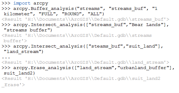
Figure 1-Data Flow Model

In accordance with Figure 1, I utilized a multitude of different spatial tools in order to determine the best place to raise a family in Austin. The tool "buffer" was imperative in creating distance radius's for the elementary schools, the parks, and the highways. Erase was important in determining the desired distance away from expressways and highways; intersect was imperative in combining all of the spatial data. Lastly, the tool "spatial join" was important in providing a summary of the total population of the inter lapped polygons that resulted from all of the buffering, erasing, and intersecting. 

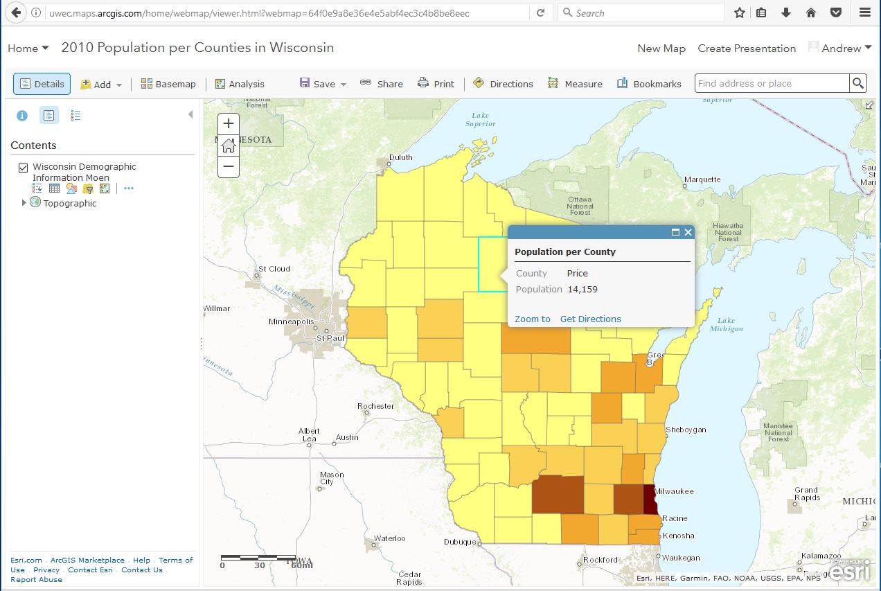
Figure 2: Map of Best Places to Raise a Family in Austin, TX

 Results: The results of the map are highlighted in Figure 2. In the map, the red lines are the highways and expressways, the gray lines depict streets; the green polygons depict parks; and the yellow polygons depict the best place to raise a family in Austin, Texas. Elementary schools, park area, and highways were depicted on the map in order to provide reference to the areas best suited to raise a family (or the yellow areas). In analyzing the map, it's noted the majority of the yellow area is located in the center of the city. This might be due to the abundance of parks located in the center of the city, and the abundance of elementary schools. There are scattered plots of yellow located in the southern and northern parts of the city; however, there seems to be a lack there of in the western parts of the city. From the looks on the map, it seems there is a lack of parks and schools comparatively on the western side of Austin, which probably explains the lack of yellow area.

Evaluation: The overall impression I had on this project was it would take all of the tools I learned this past semester in order to create both a cartographically pleasing map coupled with accurate data representation. Some of the challenged I originally faced was trying to obtain data; trying to locate data in and of itself presents a challenge, however the utilization of the "Mastering ArcGIS" data helped curtail the challenge. Also, it's acknowledged this map isn't perfect; there are some shortcomings that need to be taken into account. For example: neighborhood crime data, in my opinion, would be another important variable for families to determine where they want to raise a family. Also, the qualifications for raising a family are based on my personal preferences; other families might want different stipulations (i.e. maybe a family doesn't care they're within certain distance of an highway, or maybe they want to be within a certain distance of a pool). If I were to change this project, I might try and locate data, versus simply utilizing the Mastering ArcGIS data, because that would create a more "real-world" application to the type of GIS work I would want to do.

Lab 3: Excel, ArcTools, and Python

Goal: The Goal of Lab 3 was to become familiar with mapping a GPS MS Excel file of black bear locations in central Marquette County, Michigan, and to determine certain characteristics about where black bears were located, while also finding areas of appropriate human-based attributes in order to dictate the best possible location for a suitable bear habitat. Another goal of this lab was also to become familiar with Python coding, and how to generate a cartographically pleasing map and data flow model.

Background: Black Bears are common in central Marquette County, Michigan, and the DNR wanted to create suitable bear habitats that best suit the needs of the bears, and of the surrounding community. In order to determine the best possible bear habitats, certain characteristics about where the black bears were located needed to be examined, like what kind of forests were the black bears most apt to be located in, or whether or not they were located within 500 meters of a stream. Also, certain characteristics about the surrounding community needed to be taken account, like whether or not the DNR managed the land, and if the land was within 5 kilometers of an urban area in order to provide the best possible location for a bear habitat.

Figure 1: Workflow Model

Figure 2: Python Model

Methods: Certain methods and tools were utilized in the creation of the map. As highlighted in Figure 1, the tool "intersect" was imperative in providing overlay functions to certain feature classes, while "dissolve" was important in its ability to blend the attributes of a feature class. The tool "Buffer" was important because it provided a certain radius on a given feature class, while the tool "Erase" helped delete certain undesirable attributes of a feature class. Learning Python also helped in the utilization of the tools for the smooth enactment of the data flow model (it wasn't utilized for the model in its entirety, just the last couple of steps as highlighted in Figure 2).

Figure 3: Map of best possible locations for bear habitat

Results: The results of the map in Figure 3 suggest a couple of places for bear habitat. It was concluded that a majority of the bears were located within 500 meters of a stream, and were located in either Mixed Forest Land, Forested Wetlands, or Evergreen Forested Land. Stemming from those conclusions, it was originally calculated that the best possible bear habitats would be located in the darker green polygons. However, other factors also needed to be taken into account, like where the urban area was located and whether or not the DNR owned the land. Taking those two factors into account, the final determination for best possible location for a bear habitat is located in the yellow. It seems the majority of the yellow land is located in the central-to-north parts of the study area, with it ranging east to west. It also seems the majority of bears are also located in the central-to north part of the study area, however they don't seem to venture east as much, preferring to habit the west to west-to-central parts of the study area.

Source: Data from State of Michigan Open GIS Data --http://gis.michigan.opendata.arcgis.com/

Landcover from USGS NLCD --http://www.mcgi.state.mi.us/mgdl/nlcd/metadata/nlcdshp.html

DNR Management Units from Michigan DNR- http://www.dnr.state.mi.us/spatialdatalibrary/metadata/wildlife_mgmt_units.htm

Streams from http://www.mcgi.state.mi.us/mgdl/framework/metadata/Marquette.html

Lab 2: Shapefiles and Web Maps

Introduction: The goal of this lab was to become familiar with downloading shapefiles and attribute data off the internet in order to build maps based off the downloaded data, and to become familiar with building web maps.

Methods: The first skill learned in this lab was how do identify and download the appropriate shapefiles and attribute data in order to create maps. It was emphasized to start off on the census website to find and download the appropriate population attribute data. Once the data was downloaded, the data had to become unzipped and saved under an excel file. After the attribute data became unzipped, the Wisconsin shapefile had to be downloaded and unzipped in order to provide the spatial attributes. After the proper data was downloaded, two maps were produced: one representing the 2010 population of each county in Wisconsin, the other depicting the 2010 population percentage of citizens in each county ages 10-14 in Wisconsin.

The second skill learned in this lab was to become familiar with creating a web map. Using one of the maps created with the previous data downloaded in this lab, and also using certain arcMap applications, the map was published online on the arcMap website. Editor applications were available on the arcMap website in order to change certain aspects of the map (i.e. proper labeling).

Results: On the "2010 Population per County" map, there seems to be a greater proportion of people living in the southern part of the state versus the northern. While the greater proportion of people tend to live in the southern part of the state, it also seems the population is more concentrated toward the east-central part of the state--so a high proportion of people living in the south-east/south-central part of Wisconsin. With the "2010 Percentage of Population per County Ages 10-14" map, there seems to be no discernible spatial patterns as to which counties exhibit higher percentages of population ages 10-14. Maybe toward northern Wisconsin the percentage of population ages 10-14 is lower comparatively to the southern part of the state, however the data seems spatially scattered between high and low percentages.

This is the web map created for this lab. The "2010 Population per County" map was uploaded onto the arcGIS website for the creation of this web map. With the online map, there is the ability to use certain tools unavailable in arcMap, like the ability to click on any county and have its population come up (in this map, Price County is clicked on).

Source: The sources for these maps were the US Census for the census data, and ESRI for the base maps.

Lab 1: Becoming Familiar with Spatial Data

 Introduction: The goal of Lab 1 is to accumulate us with various spatial data sets used in public land management, administration, and land use, in order to become familiar with GIS and its applications. In order for us to understand the uses of various spatial data, we mapped the Confluence Project in relation to the various data that could correspond with its location. 

Methods: Throughout this lab, the main skill I learned was how to utilize different data in order to create six different maps of the same general area. We started off by exploring the data sets between the city and county of Eau Claire. After exploring the data, we digitized the area for the future confluence project, in order to utilize the digitization for other maps. We also learned about the Public Land Survey System (PLSS) and the legal information in order to understand the boundaries of the site, and where the site is located in accordance with the PLSS. Finally, based off the Confluence Project digitization, we created six maps that corresponded to different data in relation to the Confluence Project's location: we created maps based off of (1) the Confluence Project in relation to the civil divisions of Eau Claire County. (2) The Confluence Project based off of census boundaries and population per square mile. (3) The Confluence Project based off of zoning classifications. (4) The Confluence Project based off parcel areas. (5) The Confluence Project based off of the PLSS. And (6) The Confluence project based off of voting districts in Eau Claire.

Results: The results were six different maps of the same general area, each corresponding with a different data set. Some of the patterns with the maps emphasize the "urban nature" of the Confluence center (in the Civil Divisions map, it's evident that the Confluence center is located in the center of the city, while in the Census Boundaries map it's located in the second highest population density area per block group). The Zoning Classification map highlights the central location of the Confluence Center in accordance with the central shopping districts. In accordance with the Parcel Area map, it seems like the proposed site is larger then the average parcel area exhibited in the immediate surrounding area, while in the PLSS map the proposed site is located in the south-central part of their section. In the voting district map, the proposed site is located on the northwest side of voting district 31. 

Sources: The source for the map data is City of Eau Claire and Eau Claire County 2013, and ESRI for the base maps.